An introduction to
Deep learning
What is machine learning?
- Machine learning (ML) is a techinque which uses computers to discover patterns or information about your data.
- It is a part of the wider field of artificial intelligence
- There are lots of different types of machine learning
Examples of machine learning
- Simplest ML algorithm could be a linear regression. It automatically and iteratively looks at your data to calculate the parameters of your $y = mx + c$ curve
- A more advenced technique is K-means clustering. It is a way of finding clusters of points in your data without having to input any explicit labels.
- The most famous is neural networks (NN) which were inspired by the brain and use a directed network of connected neurons to describe features of the data set.
- More recently (since about 2010) deep neural networks (DNN) have become possible, allowing more detailed models of data to be learned starting the modern buzz for deep learning.
What are neural networks
Neural networks are a collection of artificial neurons connected together so it's best to start by learning about about neurons.
In nature, a neuron is a cell which has an electrical connection to other neurons. If a charge is felt from 'enough' of the input neurons then the neuron fires and passes a charge to its output. This design and how they are arranged into networks is the direct inspiration for artificial neural networks.
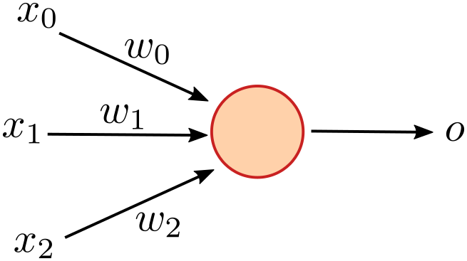
An artificial neuron has multiple inputs and can pass its output to multiple other neurons.
A neuron will calculate its value, $p = \sum_i{x_iw_i}$ where $x_i$ is the input value and $w_i$ is a weight assigned to that connection. This $p$ is then passed through some activation function to determine the output of the neuron.
Networks
The inputs to each neurons either come from the outputs of other neurons or are explicit inputs from the user. This allows you to connect together a large network of neurons:
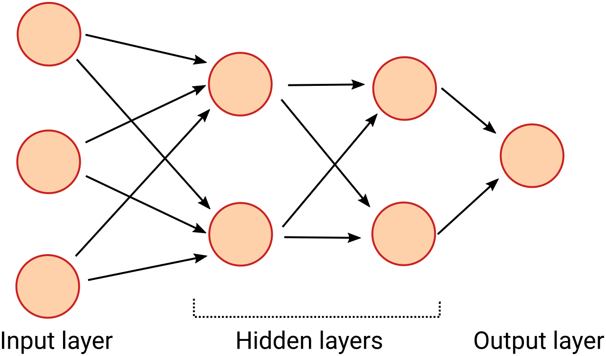
In this network every neuron on one layer is connected to every neuron on the next. Every arrow in the diagram has a weight assigned to it.
You input values on the left-hand side of the network, and the data flows through the network from layer to layer until the output layer has a value.
What shape should the network be?
There is some art and some science to deciding the shape of a network. There are rules of thumb (hidden layer size should be similar sized to the input and output layers) but this is one of the things that you need to experiment with and see how it affects performance.
The number of hidden layers relates to the level of abstraction you are looking at. Generally, more complex problems need more hidden layers (i.e. deeper networks) but this makes training harder.
How are the weights calculated?
The calculation of the weights in a network is done through a process called training. This generally uses lots of data examples to iteratively work out good values for the weights.
How do you train neural networks
The main method by which NNs are trained is a technique called backpropogation.
In order to train your network you need a few things:
- A labelled training data set
- A labelled test (or evaluation) data set
- A set of initial weights
Initial weights
The weights to start with are easy: just set them randomly!
Training and testing data sets
You will need two data sets. One will be used by the learning algorithm to train the network and the other will be used to report on the quality of the training at the end.
It is important that these data sets are disjoint to prevent overfitting.
It is common to start with one large set of data that you want to learn about and to split it into 80% training data set and 20% test data set.
Backpropogation ("the backward propogation of errors")
Once you have your network structure, your initial weights and your training data set, you can start training.
There have been lots of algorithms to do this over the last several decades but the currently most popular one is backpropogation.
The first thing you need to do is to calculate the derivative of each weight with respect to the output of the network, $D_n = \frac{dw_n}{dy}$. This gives how much you need to tweak each weight—and in which direction—to correct the output.
Then for each training entry:
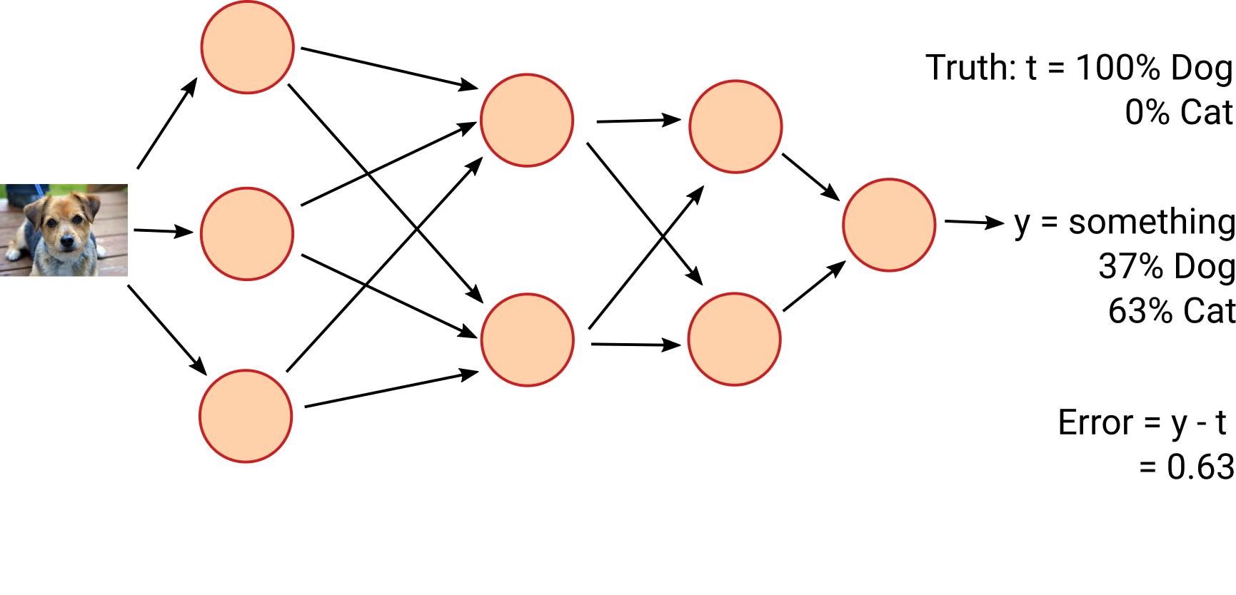
- pass it through the network and find the value $y$
- compare $y$ with the expected true output, $t$ to calculate the error $\epsilon$
- tweak each weight by $\delta w_n = \epsilon R \frac{dw_n}{dy}$ where $R$ is the learning rate
This means that the 'more wrong' the weights are, the more the move towards the true value. This slows down as, after lots of examples, the network converges.
Common neural network libraries
It would, as with with most things, be possible to to the above by hand but that would take years to make any progress. Instead we use software packages to do the leg work for us.
The can in general, construct networks, automatically calculate derivatives, perform backpropogation and evaluate performance for you.
Some of the most popular are:
- PyTorch
- TensorFlow
- Keras
- Caffe2
- scikit-learn
In this workshop, we will be using TensorFlow with a little bit of Keras.
Our first neural network: classifying Irises
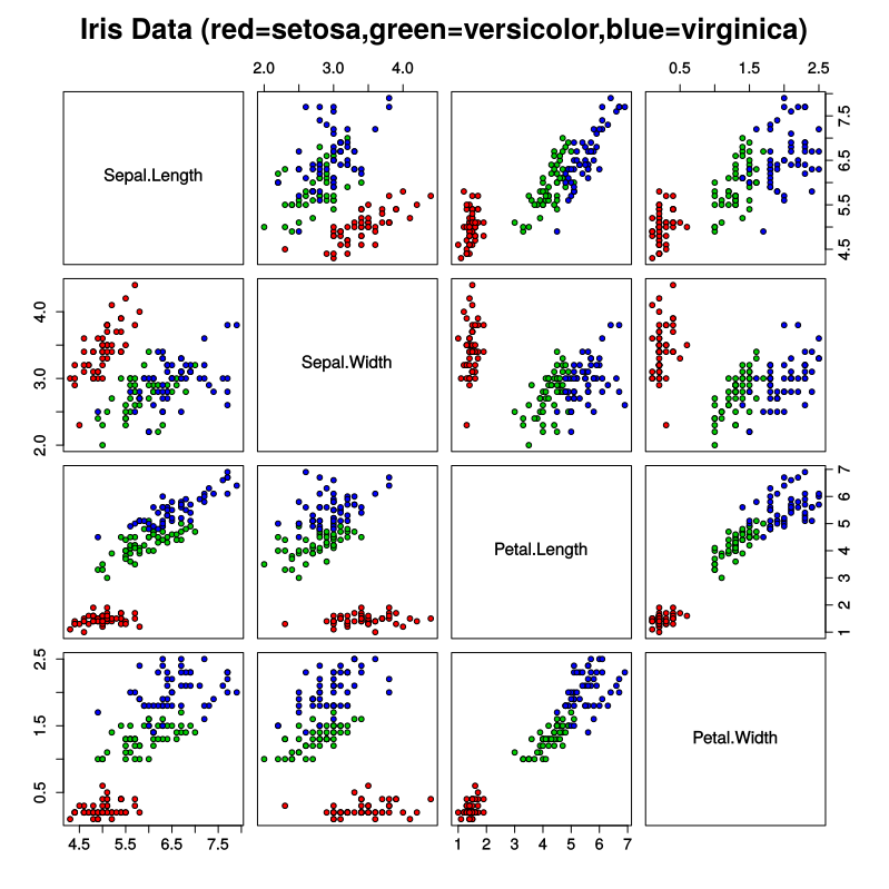
We're going to start with a classic machine learning example, classifying species of Irises.
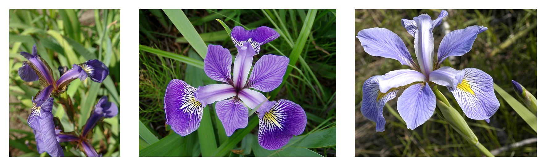
Iris setosa, Iris versicolor, and Iris virginica
Data set
There exists a data set of 150 irises, each classified by sepal length and width, and petal length and width.
| Sepal length | sepal width | petal length | petal width | species |
|---|---|---|---|---|
| 6.4 | 2.8 | 5.6 | 2.2 | 2 |
| 5.0 | 2.3 | 3.3 | 1.0 | 1 |
| 0.9 | 2.5 | 4.5 | 1.7 | 2 |
| 4.9 | 3.1 | 1.5 | 0.1 | 0 |
| ... | ... | ... | ... | ... |
Each species label is naturally a string (for example, "setosa"), but machine learning typically relies on numeric values. Therefore, someone mapped each string to a number. Here's the representation scheme:
- 0 represents setosa
- 1 represents versicolor
- 2 represents virginica
The code
The Python code that we will be running is available at premade_estimator.py. Feel free to follow along with that file but the important parts of the code will be on these slides.
Loading our data
Since we're working with a common data set, TensorFlow comes with some helper function to load the data into the correct form for us.
In iris_data.py, there is a function load_data.
>>> (train_x, train_y), (test_x, test_y) = load_data()
>>> train_x.head()
   SepalLength  SepalWidth  PetalLength  PetalWidth
0          6.4         2.8          5.6         2.2
1          5.0         2.3          3.3         1.0
2          4.9         2.5          4.5         1.7
3          4.9         3.1          1.5         0.1
4          5.7         3.8          1.7         0.3
>>> train_y.head()
0    2
1    1
2    2
3    0
4    0
Name: Species, dtype: int64
It brings in the data from a CSV file into a Pandas DataFrame.
Prepping our data
Also in iris_data.py there is a function called train_input_fn:
def train_input_fn(features, labels, batch_size):
    dataset = tf.data.Dataset.from_tensor_slices((dict(features), labels))
    dataset = dataset.shuffle(1000).repeat().batch(batch_size)
    return dataset
We pass this train_x, train_y and our wanted batch size.
- First it converts the input data format to a TensorFlow
Dataset - Then it shuffles, repeats and batches the examples
- Finally it returns the data set
Designing our network
TensorFlow comes with a network specially designed for this kind of classification problem. It automates a lot of the setup work but has a few configurable parameters.
The network is called tf.estimator.DNNClassifier (Deep Neural Network Classifier). In our case we will give it three things:
- the list of the features (in our case 'SepalLength', 'SepalWidth', 'PetalLength' and 'PetalWidth')
- the number and size of the hidden layers
- the number of output classes to create
classifier = tf.estimator.DNNClassifier(
    feature_columns=my_feature_columns,
    # Two hidden layers of 10 nodes each.
    hidden_units=[10, 10],
    # The model must choose between 3 classes.
    n_classes=3
)
and that is all that is needed to describe the shape of our network. We can now get to work training it.
Training our network
To train our network, all we need to do is call the train method on the classifier object we just created.
It takes two arguments: the first is the function to use to generate the training data set so we use our train_input_fn from above and the second is the numer of steps to perform which will change how long it trains for.
classifier.train(
    input_fn=lambda:iris_data.train_input_fn(train_x, train_y,
                                             args.batch_size),
    steps=args.train_steps
)
At this point, TensorFlow will go ahead and train the network, outputting its progress to the screen. It should take a few seconds to run.
Evaluating our model
We want to check how good a job the training did so we then evaluate our network on our test data set. It takes a very similar form to training:
eval_result = classifier.evaluate(
    input_fn=lambda:iris_data.eval_input_fn(test_x, test_y,
                                            args.batch_size))

print('\nTest set accuracy: {accuracy:0.3f}\n'.format(**eval_result))
It should print something like:
Test set accuracy: 0.933telling us that the network classified the test data set with a 93.3% accuracy.
Use the model
Finally, we want to use the model to make a prediction about the real world. Given a few examples of irises, we evaluate them using the model and compare the results to what would expect:
expected = ['Setosa', 'Versicolor', 'Virginica']
predict_x = {
    'SepalLength': [5.1, 5.9, 6.9],
    'SepalWidth': [3.3, 3.0, 3.1],
    'PetalLength': [1.7, 4.2, 5.4],
    'PetalWidth': [0.5, 1.5, 2.1],
}

predictions = classifier.predict(
    input_fn=lambda:iris_data.eval_input_fn(predict_x,
                                            labels=None,
                                            batch_size=args.batch_size))
Run it yourself
Once you are logged onto BC4, you can run the iris neural network by typing
sbatch iris.slmThat will submit a processing job to the scheduling system and will hopefully start running it immediately. It will print a number to the screen which is the job number. Make a note of this. You can check the status of your job using sacct -j 123456 (or whatever your job ID is).
Once it is finished, you can check the output using less slurm-123456.out. Press page-down to scroll through the output and q to exit. At the end you should see:
Test set accuracy: 0.967

Prediction is "Setosa" (99.8%), expected "Setosa"
Prediction is "Versicolor" (99.6%), expected "Versicolor"
Prediction is "Virginica" (98.5%), expected "Virginica"
Introduction to image analysis
The iris example worked well but the big downside is that it required manual processing of the real-world data before it could be modelled. Someone had to go with a ruler and measure the lengths and widths of each of the flowers. A more common and easily obtainable corpus is images.
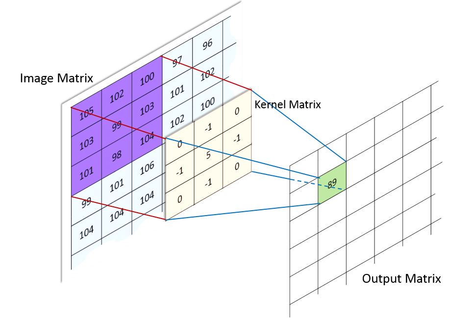
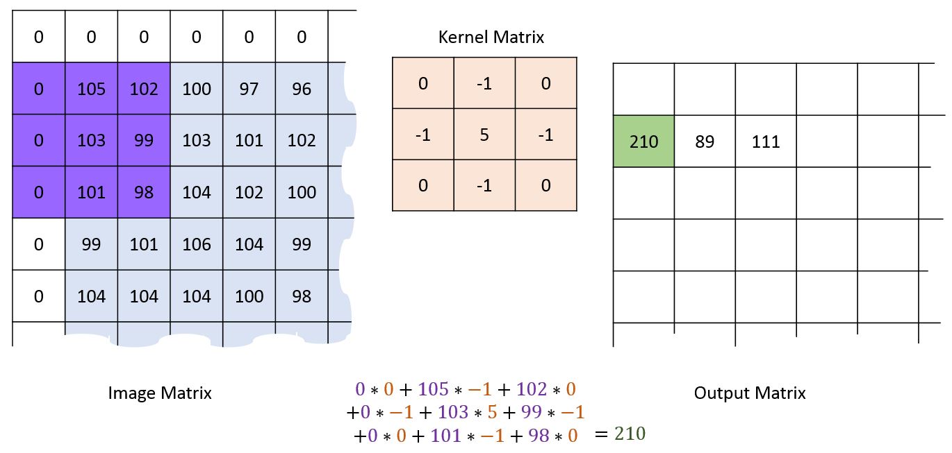
There have been many advancements in image analysis but at the core of most of them is kernel convolution. This starts by treating the image as a grid of numbers, where each number represents the brightness of the pixel
$$ \begin{matrix} 105 & 102 & 100 & 97 & 96 & \dots \\ 103 & 99 & 103 & 101 & 102 & \dots \\ 101 & 98 & 104 & 102 & 100 & \dots \\ 99 & 101 & 106 & 104 & 99 & \dots \\ 104 & 104 & 104 & 100 & 98 & \dots \\ \vdots & \vdots & \vdots & \vdots & \vdots & \ddots \end{matrix} $$Define a kernel
You can then create a kernel which defines a filter to be applied to the image:
$$ Kernel = \begin{bmatrix} 0 & -1 & 0 \\ -1 & 5 & -1 \\ 0 & -1 & 0 \end{bmatrix} $$Depending on the values in the kernel, different filtering operations will be performed. The most common are:
- sharpen (shown above)
- blur
- edge detection (directional or isotropic)
The values of the kernels are created by mathematical analysis and are generally fixed. You can see some examples on the Wikipedia page on kernels.
Applying a kernel
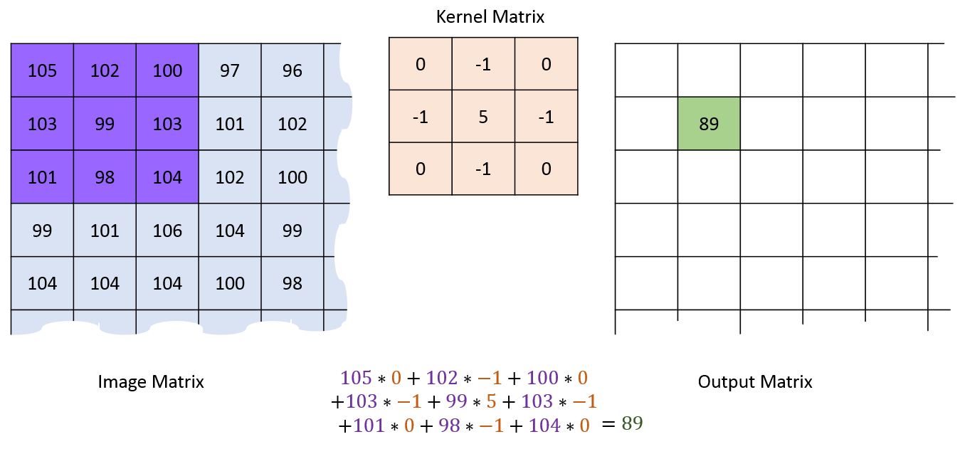
This kernel is then overlaid over each set of pizels in the image, corresponding values are multiplied and then the total is summed:
First pixel
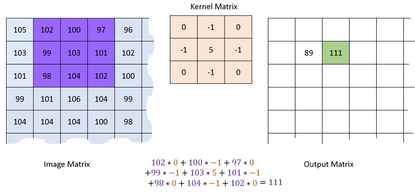
Second pixel
Dealing with edges
Convolutional neural networks
At the core of convolutional neural networks (CNNs) is their ability to create abstract feature detectors automatically. If carefully combined, you can create a network which has layers of abstraction going from "is there an edge here" to "is there an eye here" to "is this a person".
From a neural network perspective, there is little different in training. You can simply treat each element of the convolution kernel as a weight as we did before. The backpropogation algorithm will automatically learn the correct values to describe the training data set.
CNNs apply a series of filters to the raw pixel data of an image to extract and learn higher-level features, which the model can then use for classification. They usually contain three components:
Convolutional layers, which apply a specified number of convolution filters to the image. For each subregion, the layer performs a set of mathematical operations to produce a single value in the output feature map.
Pooling layers, which downsample the image data extracted by the convolutional layers to reduce the dimensionality of the feature map in order to decrease processing time. A commonly used pooling algorithm is max pooling, which extracts subregions of the feature map (e.g., 2x2-pixel tiles), keeps their maximum value, and discards all other values.
Dense (fully connected) layers, which perform classification on the features extracted by the convolutional layers and downsampled by the pooling layers. In a dense layer, every node in the layer is connected to every node in the preceding layer.
Typical CNN
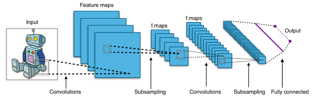
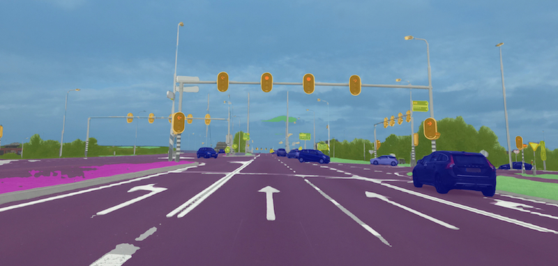
Image segmentation
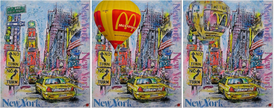
Learn painting styles
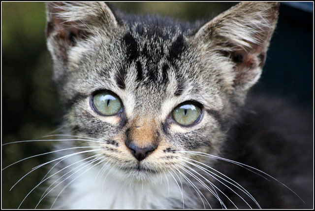
Nature
Handwriting recognition
The MNIST data set is a collection of 70,000 28×28 pixel images of scanned, handwritten digits.
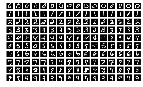
We want to create a network which can, given a similar image of a digit, identify its value.
Using TensorFow to create and train a network
In TensorFlow, there are three main tasks needed before you can start training. You must:
- Specify the shape of your network
- Specify how the network should be trained
- Specify your training data set
We will now go through each of these to show how the parts fit together.
The code we are using is available at mnist.py so feel free to have a peek but the important bits will be on these slides.
Designing the CNN
We will create a network which fits the following design:
- Convolutional Layer #1: Applies 32 5×5 filters (extracting 5×5-pixel subregions), with ReLU activation function
- Pooling Layer #1: Performs max pooling with a 2×2 filter and stride of 2 (which specifies that pooled regions do not overlap)
- Convolutional Layer #2: Applies 64 5×5 filters, with ReLU activation function
- Pooling Layer #2: Again, performs max pooling with a 2×2 filter and stride of 2
- Dense Layer #1: 1,024 neurons, with dropout regularization rate of 0.4 (probability of 40% that any given element will be dropped during training)
- Dense Layer #2 (Logits Layer): 10 neurons, one for each digit target class (0–9).
This struture has been designed and tweaked specifically for the problem of classifying the MNIST data, however in general it is a good starting point for any similar image analysis problem.
Building the CNN
We're using TensorFlow to create our CNN but we're able to use the Keras API inside it to simplify the network construction. We create a function, create_model(), which returns the definition of the network.
Reshaping the data
The first things we need to do it tell TensorFlow about the shape of our images. The data it initially gets passed is simply a 784 element long list rather than a 28×28 2D array. The Keras Reshape object can do this reshaping:
def create_model():
    l = tf.keras.layers
    return tf.keras.Sequential(
        [
            l.Reshape(
                target_shape=[1, 28, 28],
                input_shape=(28 * 28,))
        ]
    )
There are still effectively 784 input values to the network, it's simply that TensorFlow now knows how they are arranged spatially.
First convolutional layer
We then add in our first convolutional layer. It create 32 5×5 filters. Since we have specified padding='same', the size of the layer will still be 28×28 but as we specified 32 filters the overall size of the layer will be 28×28×32=25,088.
def create_model():
    l = tf.keras.layers

    return tf.keras.Sequential(
        [
            l.Reshape(
                target_shape=[1, 28, 28],
                input_shape=(28 * 28,)),
            l.Conv2D(
                filters=32,
                kernel_size=5,
                padding='same',
                activation=tf.nn.relu)
        ]
    )
First pooling layer
Next we add in a pooling layer. This reduces the size of the image by a factor of two in each direction (now effectively a 14×14 pixel image). This is important to reduce memory usage and to allow feature generalisation.
def create_model():
    l = tf.keras.layers
    max_pool = l.MaxPooling2D((2, 2), padding='same')

    return tf.keras.Sequential(
        [
            l.Reshape(
                target_shape=[1, 28, 28],
                input_shape=(28 * 28,)),
            l.Conv2D(
                filters=32,
                kernel_size=5,
                padding='same',
                activation=tf.nn.relu),
            max_pool
        ]
    )
After pooling, the layer size is 14×14×32=6272.
Second convolutional and pooling layers
We then add in our second convolution and pooling layers which reduce the image size while increasing the width of the network so we can describe more features:
def create_model():
    l = tf.keras.layers
    max_pool = l.MaxPooling2D((2, 2), padding='same')

    return tf.keras.Sequential(
        [
            ...
            max_pool,
            l.Conv2D(
                filters=64,
                kernel_size=5,
                padding='same',
                activation=tf.nn.relu),
            max_pool
        ]
    )
After this final convolution and pooling, we have a layer of size 7×7×64=3136.
Fully-connected section
Finally, we get to the fully-connected part of the network. At this point we no longer consider this an 'image' any more so we flatten our 3D layer into a linear set of nodes. We then add in a dense (fully-connected) layer with 1024 neurons.
To avoid over-fitting, we apply dropout regularization to our dense layer which causes it to randomly ignore 40% of the nodes each training cycle (to help avoid overfitting) before adding in our final layer which has 10 neurons which we expect to relate to each of our 10 classifications:
def create_model():
    l = tf.keras.layers
    max_pool = l.MaxPooling2D((2, 2), padding='same')

    return tf.keras.Sequential(
        [
            ...
            l.Flatten(),
            l.Dense(1024, activation=tf.nn.relu),
            l.Dropout(0.4),
            l.Dense(10)
        ])
Telling it how to train
TensorFlow requires that we create a function which returns an 'EstimatorSpec' which describes how the model should be trained. Here we specify which optimiser to use (ADAM is a slightly smarter gradient-descent algorithm) as well as our loss function (related to the error calculation we did earlier):
def model_fn(image, labels, mode, params):
    model = create_model()

    optimizer = tf.train.AdamOptimizer(learning_rate=1e-4)

    logits = model(image, training=True)
    loss = tf.losses.sparse_softmax_cross_entropy(labels, logits)

    return tf.estimator.EstimatorSpec(
        mode=tf.estimator.ModeKeys.TRAIN,
        loss=loss,
        train_op=optimizer.minimize(loss,
                                    tf.train.get_or_create_global_step())
    )
Creating the training data
The final thing to do before we start training is to tell TensorFlow what training data to use. We create a function which grabs the data from disk (using mnist_dataset.py), shuffles it and batches it up. It repeats the data a variable number of times ("number of epochs") before returning it.
def train_input_fn():
    ds = dataset.train(flags_obj.data_dir)
    ds = ds.cache().shuffle(buffer_size=50000).batch(flags_obj.batch_size)

    ds = ds.repeat(flags_obj.train_epochs)
    return ds
To actually start training, we create an estimator which uses our model_fn defined above and call the train() method:
mnist_classifier = tf.estimator.Estimator(model_fn=model_fn)

mnist_classifier.train(input_fn=train_input_fn)
Run it yourself
Like we did for the iris example, run:
sbatch mnist.slmAgain, it will print a number to the screen which is the job number. Make a note of this. You can check the status of your job using sacct -j 123456 (or whatever your job ID is).
Now we wait...
Check the output
Once it is finished, you can check the output using less slurm-123456.out. Press page-down to scroll through the output and q to exit. At the end you should see something like:
Evaluation results:
        {'accuracy': 0.9903, 'loss': 0.029199935, 'global_step': 6000}
...
dog. CNN thinks it's a 8 (65.2%)
1 at 5.2. CNN thinks it's a 8 (80.1%)
2 at 41.5. CNN thinks it's a 1 (55.3%)
3 at 14.6. CNN thinks it's a 8 (71.9%)
4 at 12.8. CNN thinks it's a 1 (85.7%)
5 at 99.9. CNN thinks it's a 5 (99.9%)
6 at 2.2. CNN thinks it's a 8 (86.3%)
7 at 15.8. CNN thinks it's a 1 (71.8%)
8 at 71.0. CNN thinks it's a 8 (71.0%)
9 at 0.3. CNN thinks it's a 8 (57.0%)
Or, in a more useful table form...


2 and 5 seem to have worked well but the rest are struggling.
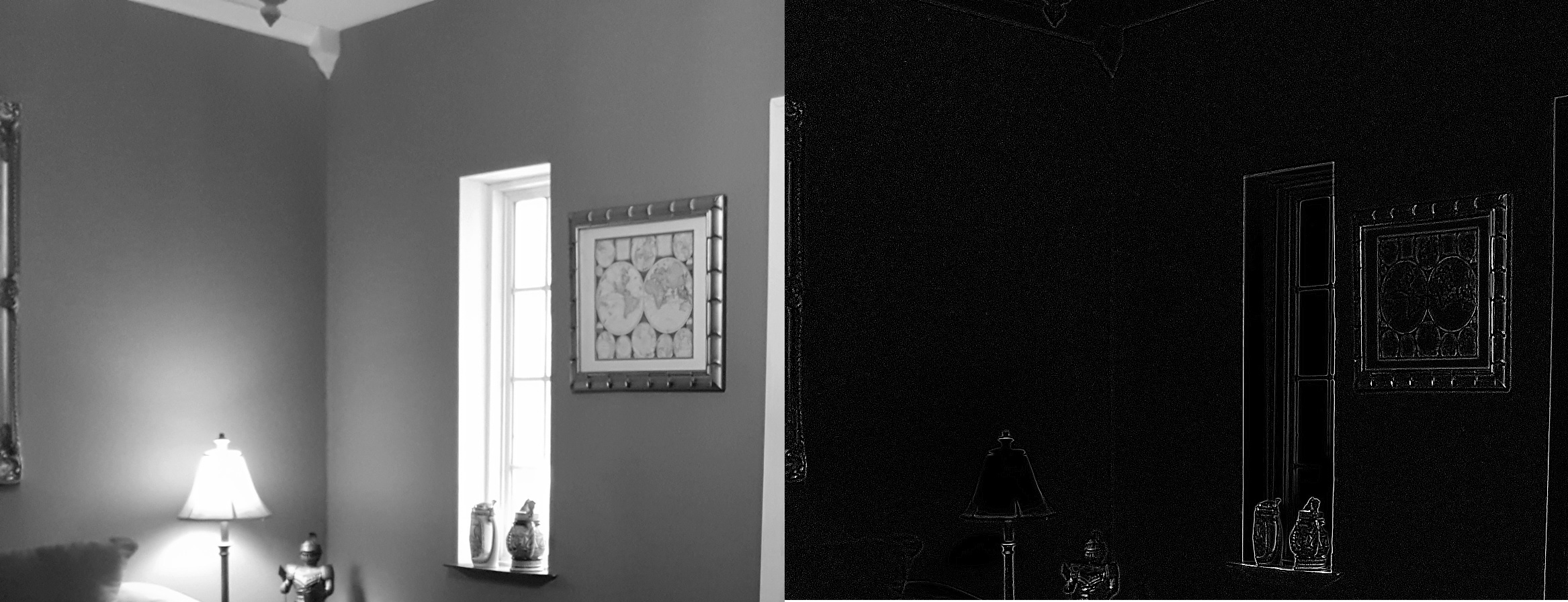
Data augmentation
The problem we're seeing here is caused by our training set being a bit restrictive. The network can only learn from what we show it so if we want it to be able to understand black-on-white writing as well as white-on-black then we need to show it some labelled examples of that too.
If you're training your network to recognise dogs then you don't just want good-looking, well-lit photos of dogs straight on. You want to be able to recognise a variety of angles, lighting conditions, framings etc. Some of these can only be improved by supplying a wider range of input (e.g. by taking new photos) but you can go a long way to improving your resiliency to test data by automatically creating new examples by inverting, blurring, rotating, adding noise, scaling etc. your training data. This is known as data augmentation.
In general, data augmentation is an important part of training any network but it is particularly useful for CNNs.
Inverting the images
In our case we're going to simply add colour-inverted versions of the data to our training data set.
We use the Dataset.map() and Dataset.concatenate() methods to double up our training set with a set of images where all the values have been inverted in the range 0-1.
def invert(image, label):
    return (image * -1) + 1.0, label

def train_input_fn():
    ds = dataset.train(flags_obj.data_dir)

    inverted = ds.map(invert)
    ds = ds.concatenate(inverted)

    ds = ds.cache().shuffle(buffer_size=50000).batch(flags_obj.batch_size)
    ds = ds.repeat(flags_obj.train_epochs)
    return ds
Run it again
Once more, submit a job to the scheduler with:
sbatch mnist_invert.slmand check the output when it is done. You should see a significant improvement.
Summary
It's possible that you only see a small improvement and even a worsening on some examples. Particularly on the 9 example, the network will struggle as it doesn't really represent the training data set. Here are some things that may improve network performance:
- More data augmentation (brightness, rotations, blurring etc.)
- Larger base training set (colour images perhaps)
- Larger number of training epochs (in general, the more the better)
- Tweak the hyperparameters (dropout rate, learning rate, kernel size, number of filters, etc.)
Ethics of machine learning
Machine learning has the problem that it can appear to be a bit of a 'black box' when processing information. You put in your question and you get out an answer. The answer isn't necessarilly correct and if you ask a stupid question (like "what handwritten digit is this dog?") you will still get an answer.
Machine learning techniques are becoming more of a part of our daily lives, used by companies to make decisions but with no human in the loop, it can be hard to challenge. Google have a set of AI principles they work towards which I recommend reading but boil down to:
- Be socially beneficial.
- Avoid creating or reinforcing unfair bias.
- Be built and tested for safety.
- Be accountable to people.
- Incorporate privacy design principles.
- Uphold high standards of scientific excellence.
Credits:
- Dog photo: CC BY 2.0 Emily Mathews
- Irises: Iris setosa (by Radomil, CC BY-SA 3.0), Iris versicolor (by Dlanglois, CC BY-SA 3.0), and Iris virginica (by Frank Mayfield, CC BY-SA 2.0).
- Kernel convolution images: http://machinelearninguru.com/computer_vision/basics/convolution/image_convolution_1.html
- CNN layout: CC BY-SA 4.0 Aphex34
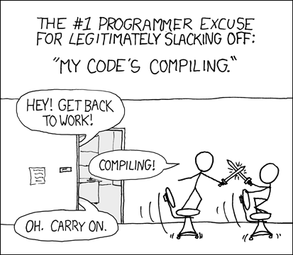
- XKCD Compiling comic: CC BY-NC 2.5 Randall Munroe
- Image segmentation: Copyright Mapillary
- Deep painterly: Fujun Luan