Numpy and Simulations
In [1]:
%load_ext interactive_system_magic
decay.py
import numpy as np


def initialise_state(num_steps, initial_value):
    """
    Args:
        num_steps (int): the number of iterations to run the simulation for
        initial_value (float): the value to start decaying from

    Returns:
        np.array: a container for the system state with the initial state present
    """
    state = np.zeros(num_steps)
    state[0] = initial_value
    return state


def update_state(old_state):
    """
    Args:
        old_state (float): the previous value

    Returns:
        float: the value, decayed
    """
    DECAY_RATE = 0.9
    new_state = old_state * DECAY_RATE
    return new_state


def run_simulation(num_steps, initial_value):
    """
    Runs the simulation using the rules defined in ``update_state``.

    Args:
        num_steps (int): the number of iterations to run the simulation for
        initial_value (float): the value to start decaying from

    Returns:
        np.array: the overall state for the system
    """
    state = initialise_state(num_steps, initial_value)

    for t in range(1, num_steps):
        state[t] = update_state(state[t-1])

    return state


INITIAL_VALUE = 100
NUMBER_OF_STEPS = 100  # Set this to 100

value_history = run_simulation(NUMBER_OF_STEPS, INITIAL_VALUE)

np.savez_compressed("decay", state=value_history)
$
python decay.py
We can then load the data and plot it. We can do this either in a Jupyter Notebook cell or in another python script:
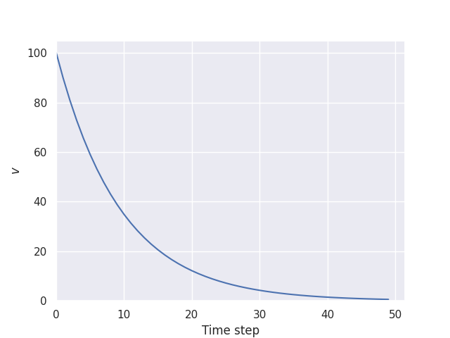
decay_plot.py
import numpy as np
import seaborn as sns

sns.set_theme()

with np.load("decay.npz") as f:
    value_history = f["state"]

g = sns.relplot(data=value_history, kind="line").set(
    xlim=(0,None),
    ylim=(0,None),
    xlabel="Time step",
    ylabel="v"
)

g.savefig("decay.png")  # Save the graph with this line
$
python decay_plot.py
This has created a file called decay.png: